PCA State Space Analysis
I’ve made progress in plotting the motion-corrected video data in a reduced high-dimensional space using PCA. Building off of my previous blog post, here’s what I’ve done to preprocess the data:
take data with the dimensions (y_pixel, x_pixel, samples) and perform the following preprocessing: 1) Flatten the first two dimensions - y and x dimensions in y_x 2) Load the behavioral data (ie. stimulus onset times) 3) Calculate a vector of samples that encompass a trial’s window 4) Make a matrix of those sample vectors across trials and extract fluorescence data using those sample indices 5) Average across trials and conditions to get a matrix of (pixels, trial_samples)
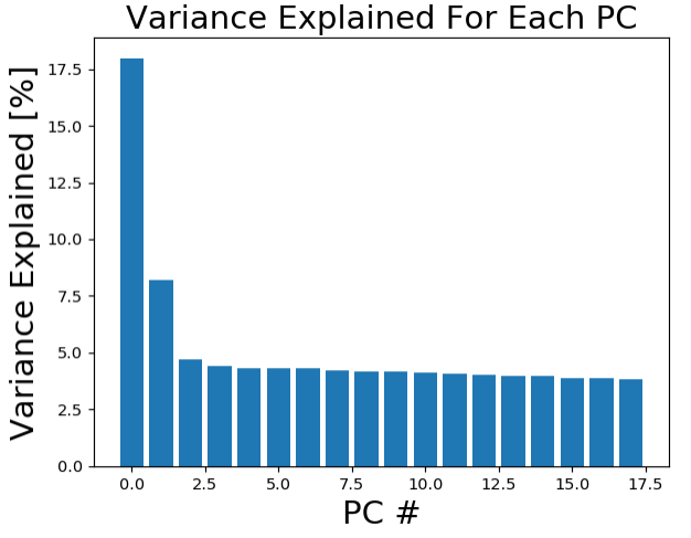
These data are then used to fit a PCA model. Here are the top principal components that explain 90% of the variance:
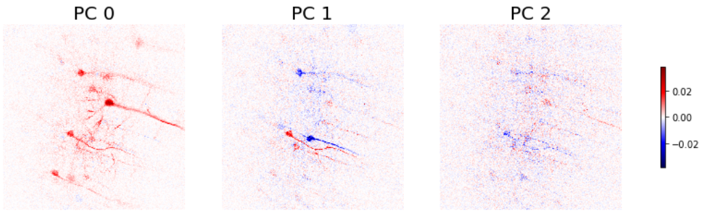
Here are the eigenvectors for these principal components reshaped to the dimensions of the recordings:
Now one way to examine which principal components contribute to the video across time and how is to create a 3D plot with the axes as the top three principal components. Then the traces traversing through this new space represent “activity” across trial time. Here are the code snippits to do so:
from mpl_toolkits.mplot3d import Axes3D
from mpl_toolkits.mplot3d.art3d import Line3DCollection

# Create a set of line segments
points = np.array([x, y, z]).T.reshape(-1, 1, 3)
segments = np.concatenate([points[:-1], points[1:]], axis=1)

# Create the 3D-line collection object
lc = Line3DCollection(segments, cmap=plt.get_cmap(cmap),
                    norm=plt.Normalize(np.min(color_encode), np.max(color_encode))) # set LUT for segment colors
Where x, y, z are the time-series for the top three components from PCA.
# create plot and set attributes
fig = plt.figure(figsize = (9,7))
ax = fig.gca(projection='3d')

ax.add_collection3d(lc, zs=z, zdir='z')
Here’s when I project the trial-averaged activity time-series for each condition into the space. CS- trial average trace starts red (-1 seconds relative to cue onsset) then ends in a yellow color (3 seconds after cue oneset). The CS+ trial trace starts blue then ends green.
To see how trials across the course of the session evolve through this high-dimensional space, I averaged trials in groups of 10 across the session and plotted them into the space. Trial block is encoded by alpha.
Check out the Jekyll docs for more info on how to get the most out of Jekyll. File all bugs/feature requests at Jekyll’s GitHub repo. If you have questions, you can ask them on Jekyll Talk.